Temperature Measurement with PT100 or PT1000 Platinum Resistors

Circiut using an IC, designed for a temperature measurement with Platinum Resistors PT100 and PT1000.

Introduction:

The number of IC components, the temperatures to measure know very strongly rose. The attainable accuracies are considerable. Accuracies smaller a degree create very many IC's. The number of components grows constantly, the components more inexpensive, smaller and will have a reduced power demand Most temperature components integrated the actual sensor element in the housing, the diode voltage of an internal transistor were in most cases measured. With negative temperature coefficients of the diode voltage the temperature is determined. Predivide this principle are combined the small costs with minimum space requirement.

any wish?

Yes, this: Disadvantage of the IC's with integrated sensor element is the reduced temperature range. It will not exceed 55°C to approx. 125°C in the best cases, since the IC is exposed to the ambient temperature. The measurement with PT100 or PT1000 platinum resistance is a special task, here is the sensor element (platinum resistance) and evaluation electronics from each other spatially separably. Electronics can evaluate the platinum sensor without high temperature fluctuations. A platinum sensor can measure a temperature range from -200 to +850 degrees (surely existing special solutions, which can do more).

A further advantage is that platinum sensors are available in the most diverse designs, with thread. Totally enclosed variants to withstand over the most diverse chemicals or very small held for miniaturized applications. It is also favourable that platinum sensors flowed through only from a direct current. A digital sensor on processor basis has principle-causes a clock rate mostly in MHz range, this clock can disturb neighbouring sensitive circuits. A platinum resistance with direct current disturbs neighbouring sensitive circuits only insignificantly. A main advantage of the platinum sensors is naturally the very high linearity of their resistance vs. temperature, a good basis for precise measurements.. NTC resistances (N negative T temperature C coefficient) are substantially nonlinear in addition, more inexpensive than their colleagues from platinum. Still another temperature sensor from the group "separately from evaluation electronics", are the thermocouples, which have a very large measuring range.

For all three groups (platinum, NTC and thermocouples) particularly for it developed evaluate IC exist. Let me show a complete circiut with the IC good for PT100 and PT1000 platinium sensors.

Part is obsolete.

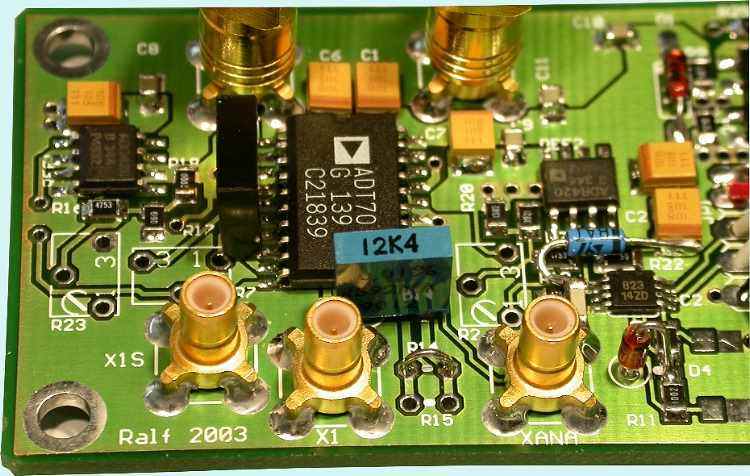
The printed circuit board shows the IC in the center, on the left and on the right of it a reference and down right a AD converter. The blue 12k4 is a resistance with 0,01% tolerance and smallest TK, the black same with 1000 ohms. The plugs serve for fast connecting of different platinum sensors in four wire connection. Completely on the right side is a discrete very fast voltage regulator. The circuit is developed for a 5-7 V single power supply. The schematic diagram is to be taken from the IC data sheet, the majority was taken from there. The circuit was adapted to the boundary conditions of the targeted application. For example also a digital output had to be placed at the layout, therefore the AD converter. The temperature range which can be measured is adjusted to -100°C to 100°C. The blue Schottky diode is a forgotten "fear diode", which was later soldered at this prototype. For trimming three potentiometers were inserted, which were replaced after successful trim by fixed resistors. These potentiometers are meaningful also if the sensor must often be exchanged and everyone of the new sensors must be trimmed.

It does not make here a sense the connection diagram of the above circuit to show exactly, for Analog Devices describes the circuit very in detail, and an adaptation to the own boundary conditions is always necessary from experience.

Theory of Operation?

The IC has two inserted precision current sources of typically 900 µA. The special is that both current sources supply almost same current, with a typical mismatching of 0,5µA to each other. One additional poti cancel out this mismatching. One of the two current sources supplies a precision resistance of 1000 ohms, with a voltage drop of 900 mVs. The second current source feeds the platinum sensor, in our case a PT1000, a platinum resistance, that has at a resistance of 1000,0.. Ohm has (in the ideal case). At both resistors the same voltage drops with zero °C. An integrated instrumention amplifier amplifies the difference voltage drop at both resistors. With zero °C, the difference would be in the ideal case zero ohm.

Differencies between PT1000 and PT100

A PT1000 is however a temperature-dependent resistance. It has 1000 ohms with zero °C, with 1°C 1003.85 ohms with 10°C 1038.5 ohms and so on. The temperature coefficient amounts to depending upon platinum material +3.85 Ohm/°C with the PT1000 and +0.385 Ohm/°C with the PT100. A PT1000 has therefore a larger slope and makes possible thereby a higher resolution. The sensor has small currents, a self-heating of sensors small is minimized. With a PT100 it is easy to develop thermometers for a large temperature range.

Closed loop of the differential amplifier sets the measurement range

We know now the voltage drop at the precision resistance remain constant, the voltage drop at the platinum sensor rise with increasing temperature and concomitantly the difference at the instrument amplifier. The instrument amplifier amplifies this difference with a fixed gain. The gain can be adjusted through external resistors. The gain factor determines the measuring range. It is obviously a measuring range from -200°C to 800°C reached naturally not the dissolution as for example -50°C to 50°C. All details in addition are located in the data sheet. In principle the circuit can be copied from single components. A question whether it is worthwhile itself.

Important Note

Circiut for single and dual supplies
PT100 or PT1000 usable
take care for the type of the platinium, if Europian or US, details in the IC datasheet and in the sensor datasheet
use the sensor datasheet, manufactorer calculate a polynom to correct the nonlinearity of the sensor
Thermocouple voltage errors
Four wire connection for precise measurements
Layout, power supply and shielding
Calibration neccessary for a high accuracy

Calibration

for calibration the ideal suitable aids are a voltage meter, an exactly well-known reference temperature (exact thermometers) and easily adjustable precision resistance decade as well as a computer. A tolerance of 0,01% for the decade would be fine.

With one of the three trimmers the sensor tolerance of 1000Ohm can be adjusted. In addition the momentary ambient temperature is accurately measured. With the voltmeter measure the output voltage at the IC, must they be adjusted to the desired value of the pertinent temperature. A platinum sensor with high basic accuracy is not necessary, because of the manual calibration. The linearity would have to be similar even with lower-priced copies, as with one with high basic accuracy, whereby I am not at all times so safe there - please consider sensor data sheet. With the last of the three trimmers the amplification of the instrument amplifier can be adjusted, whereby that is the most important attitude.

With the decade now the different temperatures can be simulated, you need therefore no climatic chamber. Measuring over the entire temperature range and the representation as graph are very useful. Unfortunately also you will state that this requires several iterative runs, until you achieve an acceptable result. In particular adjusting at the rotary buttons difficult to operate of the decade costs nerves. Sometime if you your desired temperature range is exactly enough should you thereby stop. In this phase you can turn at the potentiometers as you want, nothing happens what you expect - a potentiometer affects the other one with a reciprocal effect. Besides the influence of the non-linearity of the sensor becomes more largely, in particular with temperatures far away from the zero point. Unfortunately the curve continues to run away always.

Now only the computer calibration helps. Finally you always wrote the measured values, or still better directly in a PC mathematics program wrote. Polynomial correction for the linearization of the measuring curve, afterwards it is correct also over the entire temperature range. With applications with a computer (AD transducer) a polynominale involution (correction) should not be an obstacle.

Ice water and a clinical thermometer

In order to know at least two points of the PT1000 characteristic, also physics helps. Who does not have a resistance decade available and precision thermometers, can do it with ice water and a clinical thermometer. These should have an accuracy in the order of magnitude of 0,1°C. Sensor attach at an ohm meter and together with the thermometer under the axilla, approx.. 10 minutes wait to took place a thermal reconciliation. In order also the self-heating of the platinum sensor ideal-proves to consider, can be operated the sensor also from the current source. This method required however additionally very a precise measurement of the small current, that is not a cheap measuring instrument, suitably e.g. a HP 3457A. The ice water method is based on the fact that with normal air pressure melting ice water has a temperature of zero °C. The water should be constantly agitated thereby. Even I tried still none out of the methods.

Table of the resistance of a PT1000 platinum sensor vs. temperature

Graph shows the calibrated result in comparison with and without AD-Converter

The graph shows the calibrated circuit, in the comparison the similar voltage with the digitized value of the AD converter. The circuit was so far trimmed that that uses usually range becomes optimum, here -10°C to +70°C. To mark is, here is not yet end of workday. The upward gradient of the instrumention amplifiers characteristic is not yet completely optimized. Only in order to repeat it again, in this stage of the calibration it is an iterative process at all three trimmers, and it became sometime me too boringly, since I had concentrated on the frequent use range and deeply into cold weather go only rarely. If you correct for example the upward gradient better, then it can push the whole curve upward or it turns around the zero point etc.. Here can be spent infinitely much time.

The triangle develops because the sensor manufacturer in the table only integral ohms of values indicated, what happened for reasons of the simplification. From the missing tenths this quantized appearance of the characteristic results. In reality the characteristic runs naturally centrically through by the triangle. Me met steps of five °C Celsius. From these measured values it would be to be accomplished now simply polynomial a correction, which would as far as possible linearize the characteristic in the PC.

I am content also with the result 12 bits. Twelve bits correspond to 4096 discrete stages. Divided for a measuring range of +-100 °C a digital dissolution of approximately 0.05 results °C/Bit, which should be sufficient. The digital measured value with 25°C I must times more exactly regard, the point fit myself not the result. A transmission or a measuring error? The converter?, it requires a renewed investigation.

normalized

The zero voltage corresponds to the reference voltage. In the table it was normalized on it.

The table shows the resistance in ohms of a PT1000 as a function of the temperature in °C as well as the output voltage of the printed circuit board. The output voltage normalized with the output voltage value, which is to appear with zero °C.