7L5 Spectrum Analyzer

The Tektronix 7L5 is an easy to operate Spectrum Analyzer with a capability of 20 Hz to 5 MHz (full range).

• Resolution bandwidth can be varied from 10 Hz to 30 kHz in a 1 - 3 sequence, residual FM of no more than 1 Hz peak-to-peak. 
• Digital storage allows a very comfortable viewing under long sweep setting 10 seconds to 100µs and an Auto-Function in a 1 -2 -5 sequence.
• Digital averaging and peak detection, one can accurately measure low level signals, such as intermodulation, distortion products in the presence of noise,
• Max Hold-Function allows capturering short duration and transient phenomena, otherwise they will be lost.
• Easy-to-use three knob operation - you set frequency span, center frequency, reference-level all other settings are set automatically.
• Digital tuning and synthesizer
• six-digit digital readout, illuminated frequency marker dot in the CRT, fine tuning selectable
• Square Wave Output Calibrator 500 kHz, -40dBV amplitude
• Reference level in 10dB and 1dB steps
• 80 dB spurious-free display dynamic range
• calibration selectable in dBV or dBm

This instrument is a nice general purpose instrument for many applications within this frequency range. Should operate in every (I am not 100% sure) 7000 series mainframe using the right vertical and the left horizontal compartment. Good choices are the mainframes 7704A or the 7603 with the extra large 1.22cm/DIV CRT for a very comfortable viewing.

There were different input modules and options available:

• L1 --- fix 50 ohm
• L2 --- fix 75 ohm
• L3 --- switchable 50 ohm, 600 ohm or 1 Mohm.
• L3 Option 01 --- switchable 75 ohm, 600 ohm or 1 Mohm
• Option 25 --- Tracking Generator sweeps 20 Hz to 5 MHz
• Option 12 --- 7854 waveform oscilloscope compatibility

It's difficult taking photos from this Plug-in, the electronic is buried under the shields.

Spectrum Analyzer's Calibrator Output:

Spectrum Analyzer -40dBV, 500 kHz Calibrator signal, 7L5 operating in a 7704A mainframe.

CRT Readout shows the analyzer settings:

•  -40 dBV Reference-level, here set to the top graticule
• 10dB/Division
• Resolution Bandwidth 30kHz
• Frequency Span 500 kHz/Division
• Illuminted dot can be moved with the DOT MKR knob for a precise frequency readout (this newly Plug-in need a readjustement of the dot position, has a small frequency offset).

Mainframe Calibrator Output:

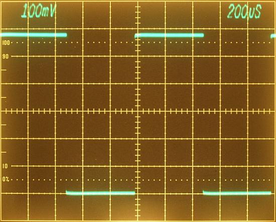
7704A mainframe 1kHz calibrator output (4V terminated with 75 ohm)



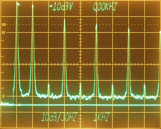
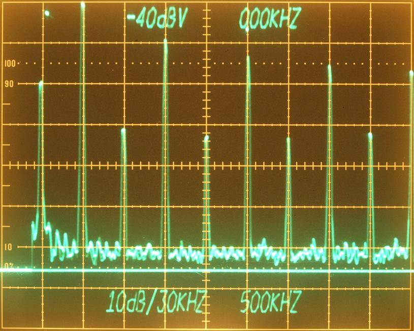
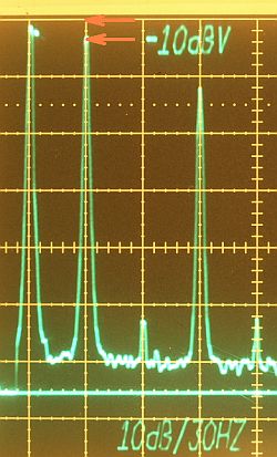
Spectrum Analyzer Measurement of the mainframe calibrator

A sunday evening calculation,

and a human eye scan of the CRT magnitudes.

Jean Baptiste Joseph Fourier would be happy see people doing such experiments, he could not do it 200 years ago. You never know if he will browse these site in the internet, I don't know if they have a line there, I have enough time to know, later.

spectral line	harmonic description	harmonic order	measurement, rms value from CRT	conversion in rms volts 10 exp (x/20)	ideal Fourier coefficient (fraction)	ideal Fourier coefficient (decimal)	measured Fourier coefficeint (conversion rms/fundamention rms)
1 kHz	fundamental		-13 dBV	224 mVrms	1	1.0	1.0
2 kHz	2. harmonic	even	negligible		-
3 kHz	3. harmonic	uneven	-22 dBV	79 mVrms	1/3	0.333	0.352
4 kHz	4. harmonic	even	negligible		-
5 kHz	5. harmonic	uneven	-25.2 dBV	55 mVrms	1/5	0.2	0.245
6 kHz	6. harmonic	even	negligible		-
7 kHz	7. harmonic	uneven	-27.8 dBV	41 mVrms	1/7	0.142	0.183
8 kHz	8. harmonic	even	negligible		-
9 kHz	9. harmonic	uneven	-29 dBV	35 mVrms	1/9	0.111	0.156

 

Conversion from rms in the fundamental amplitude, A = 224mV * 1.4142 = 317mV

Fourier series of an ideal (no DC-component) square wave: y(t) = 4*317/Pi  * [sin(wt) + 0.333*sin(3wt) + 0.200*sin(5wt) + 0.142*sin(7wt) + 0.111*sin(9wt) .....]
              Fourier series of the measured CRT square wave: y(t) = 4*317/Pi  * [sin(wt) + 0.352*sin(3wt) + 0.245*sin(5wt) + 0.183*sin(7wt) + 0.156*sin(9wt) .....]

with w=2*Pi*f


A quick browsing tour in the internet take me to a website offering an freeware function plotter tool called Mathegrafix



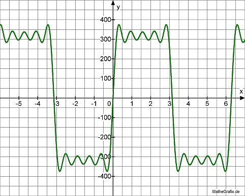
square wave with ideal (green line) Fourier 9th. order coefficients




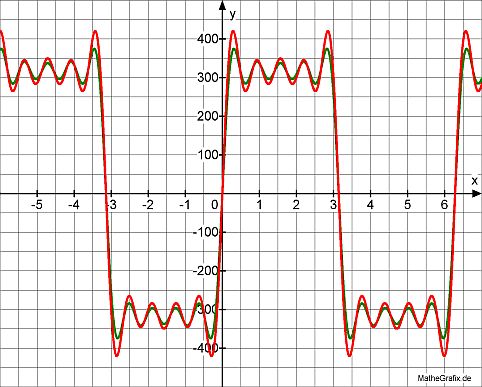
square wave with measured (red line) Fourier 9th. order coefficients overlayed to the ideal (green line) waveform

Overlaying Pictures:

Overlaying with software for an easy comparison between scope and analyzer  measurement.
    
square wave calculated with the measured Fourier coefficients                                      square wave signal measured with the oscilloscope




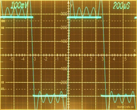
Overlaying of measured Fourier coefficients (9.th order) with the oscilloscope, (both diagrams using the same vertical scalefactor).


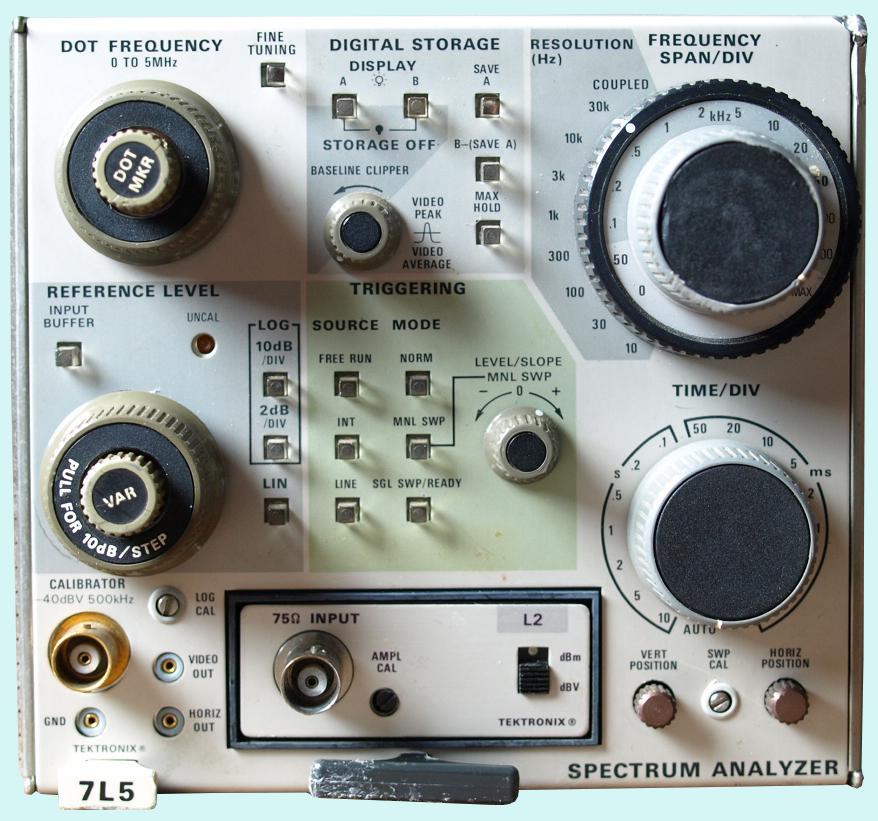
Let me say the spectrum analyzer works very well, I got the instrument newly and I have not yet calibrated the instrument following the calibration procedure in the service manual.

Some minor measurement errors:

by the time I did the oscilloscope photo I never planed to do a sunday evening calculation, let me explain the small amplitude difference between the Scope and Analyzer measurement. It's difficult to read the exact spectral length with the eye.

    

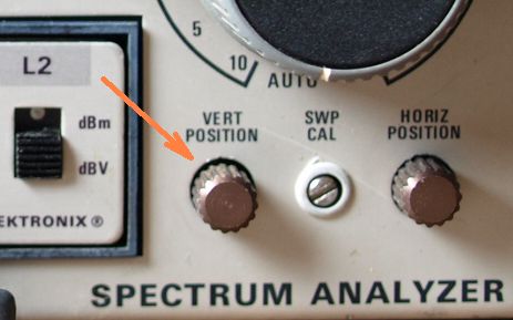
Before I took the photo I haven't measure the real distance between top graticule (-10dBV reference level) and a 1 kHz sine wave with known amplitude. Before doing an accurate amplitude measurement you should calibrate the setted reference level position. Now the reference level depends on the position of the VERT POSITION control and this will cause a deflection error in the fundamental wave.

In this measurement the reference level wasn't perfect adjusted, you see the small amplitude diffence between the calculated and the calibrated square wave in the overlayed photo. The amplitude ratio of the fundamental and the harmonics is correct, their ratios were derived from the distance between fundamental and the harmonics, if occurs wrong ratios would have their reasons in a wrong analyzer vertical deflection gain.

When using an spectrum analyzer Plug-in be sure that the mainframe has a correct adjusted vertical gain and geometry.  One should know the oscilloscope vertical linearity, special a non-linearity in the top graticule area cause high amplitude errors because the analyzer use in most cases the LOG scaling !!!, this is important to consider, because many not well adjusted CRT geometries suffer in the outer vertical top and/or bottom  areas.

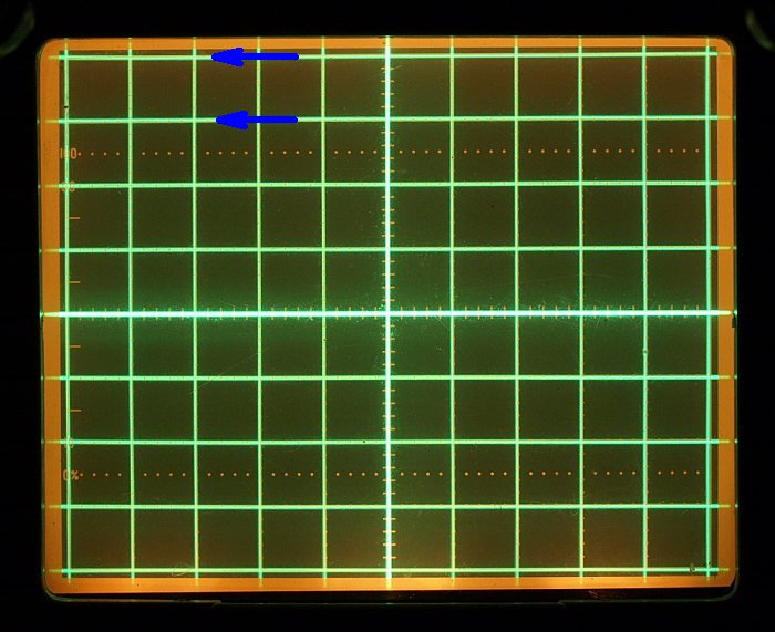
This is an example for a well adjusted CRT geometry and a correct vertical gain. Be sure that the analyzers mainframe has a proper adjusted vertical gain in the blue arrows area. The photo is taken from my 7844, for the used 7704A I took not a photo during calibration. If calibration fixtures were not available, the vertical top graticule linearity can be tested in a simplified manner with a one division square wave moved up and down with the plug-in amplifier offset control.

Have fun with this nice Spectrum Analyzer