Slew Rate

The slew rate is an important characteristic for amplifiers and electronics of elements

Introduction

The slew rate is comparably with a speed, in this case e.g. the temporal change of a voltage or an electric current. This term is admits from classical physics, a body moves with for example with 5 meters per second. In electro-technology the slew rate developed, for example a voltage changes its level within a certain time, defined in the unit volt per second in analogy.

Comparison from the everyday life

Already with a simple comparison of the slew rate of two amplifiers, first statements can be met from this parameter. A car or a motorcycle with a maximum speed of 250 km/h is clearly faster than one with 120 km/h. Simplified said, the slew rate is the maximum speed of an amplifier. Alone the maximum speed does not say yet much about applications and qualities of a vehicle. With a vehicle with a maximum speed of 250 km/h no truck may be expected. Do not ask - with a Slew rate of 4000 V/µs a Hifi amplifier output stage to expect is utopian, the inaugurated electronics engineer thinks thereby immediately of video operation amplifier or similarly fast parts

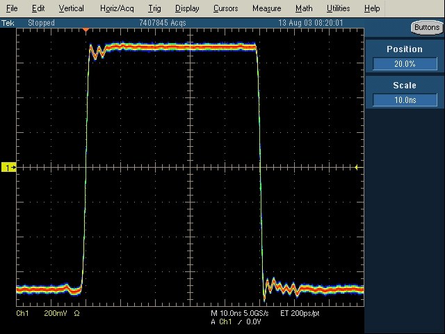
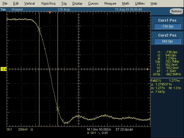
Figure 1 shows a 10 MHz square wave signal of a Tektronix AWG430 generator. Measured with a Tektronix TDS5054 oscilloscope with a rise time of approx.. 800 picoseconds. At the scope a multi-color mode is adjusted, in order to represent the intensity of the "electron beam" better. Time base 10 ns/DIV, vertically 200mV/DIV. 50 ohms.

The picture shows that also very good generators are not yet perfect. A settling time and a finite slew rate will be always present. The figure shows that even a very good generator is still not perfect. A remaining settling time and a finite slew rate. The desired "rights angles" there are not in nature and it will not also give, only in mathematics. For measuring the Slew rate the optimum rectangle and fastest oscilloscope should be used, which are available. In particular with very fast operation amplifiers this is particularly important. For a Hifi amplifier is strongly reduced the requirement to the speed of test equipment, because of the lower speed of audio devices.

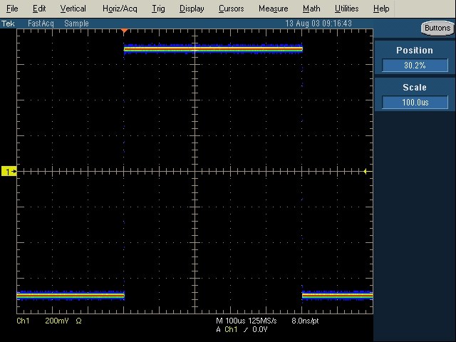
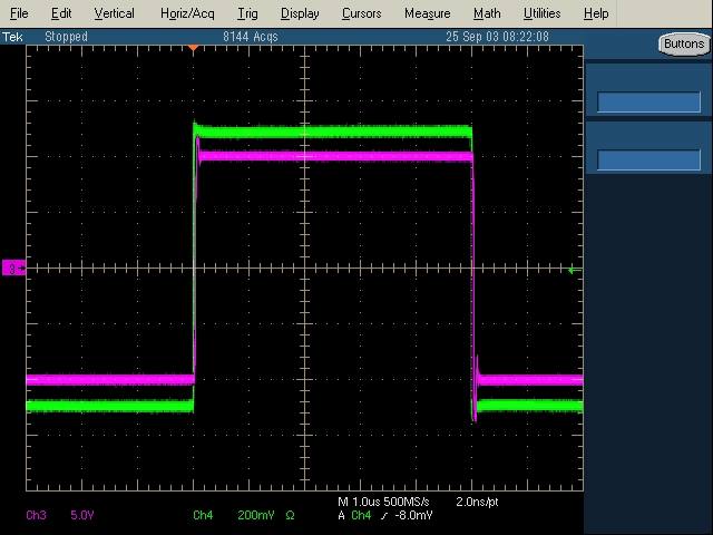
Figure 2 shows the same test tequipment, now however a 1 kHz square wave signal. Meanwhile this signal on the oscilloscope looks perfectly. A settling time are not to be recognized visible with this time base. For a audio amplifier is 1 kHz signal a good choice, the primary wave (1 kHz) and also still many rectangle harmonic waves (3, 5, 7, 9 kHz etc..) are appropriate still within the audio range and can be transferred by the amplifier. To put on a 10 MHz square wave signal to a hifi amplifier would be senseless, it is the developer would like to know whether the amplifier reacts to higher-frequency signals with oscillation at the output.

It is forbidden that with a Slew rate measurement a loudspeaker is attached, since the tweeter is destroyed by the high frequencies and levels. 

For a test a level is recommended, approx.. 5% to 10% under the maximum output voltage with normal load (e.g. 4 ohms).

Figure 3 is the same signal as in fig. 2, only oscilloscopes shows the signal in another representation method. The multi-colors mode is switched off and the "digital electron beam" stands on green, and shows like the square wave signal on a similar oscilloscope would look. To see also here, a minimum oscilloscope noise. A analogue oscilloscope is just as well suitable for the measurement of the Slew Rate as a digital.

Figure 4 shows the rising edge of 1 kHz square wave signal. The rise time usually measured between 10% and 90% of the amplitude. Comfortable way computes the oscilloscope the rise time with 1.578 nanoseconds. The Slew rate of this signal amounts to 709.8 megavolt per second. Converted into the usual Volt/µs results in: 709.8 V per microsecond. The analog scope user must count the division lines of the scaling and accomplish the calculation of the delta y by delta x. The true square wave signal is still faster, since that oscilloscopes adds approx. 800ps. Such a rate of rise of the testsignals is already more than sufficient for a Hifi amplifier. To see very beautifully the clean settling square wave signal with very small overshooting, this are from similar nature as in fig. 1.

Figure 5 shows the falling edge of 1 kHz of square wave signal. The Slew rate became negative now, since the voltage sinks. The oscilloscope computes -862.5 V per microsecond. The falling edge is faster than the rising edge. With these small times is however tolerable. Ideally it would be natural if both were alike. To observe beautifully that the flanks are from more clearly very symmetrical nature. That speaks qualitatively for the measuring instruments.