Comments on Figure 1
Bandwidth only 35 kHz
that means an early voltage drop for high signal frequencies, which lie
still in the audible range. Result is a smaller amplitude for this signal
frequency. We go once of it out of the developers a theoretical
reinforcement of 40dB had aimed at, in the range of 20 kHz reach it only
38,2dB. As relationship expressed: 40/20 and this quotient in the
exponents to the basis of 10 sets, results in 100. The amplifier
strengthens thus maximally with factor 100 in the desire conception.
However 1,8dB are missing to it to the ideal value. DB's can be reckoned
back again: 1,8dB/20 and this quotient in the exponents to the basis 10
set, there come out a number of 1,23. 100/81.2 = gain error ratio of 1.23
What does it matter 1.23?
it is the gain error ratio. Let's have a look at
figure 3, we define the maximum input to exactly 150mV, the output should
be 150mV * 100 =15V at 20kHz. Unfortunately there is an error 15V / 1.23 =
12.2V instead of 15V.
Short calculation for influence on power:
Ptarget = 15V*15V / 4 ohm = 56.25 Watt
Pnow = 12.2V *12.2V / 4 ohm = 37.21 Watt
Sorry, 56.25 Watt - 37.21 Watt = 19.04 Watt missing output power at
20kHz.
Very nice?
|
Comments on Figure 2
Twisted Amplitude Response
the frequency response should be smoothly like a ruler over the entire
audio range and sufficient in addition it. Following the writing in the
left column, the equations can be applied naturally also 1:1 to the entire
amplifier frequency response . Optically clearly recognizable statement,
the amplifier is clearly violently stressed in the range upper bass and
the mid range. The amount of the deviation is not tolerable. Can this
error be corrected by adjusting at the bass and treble control? My answer
to it: the sound controllers stood during the measurement accurately in
mid range position. Is it now actual the task of the customer to correct
by means of complex measuring technique the work of the developer again?
Probably hardly. I naturally tried it. The curve can be improved, it
becomes bent for it however again with other frequencies.
Reasons for these nonlinearity?
is to be said only with difficulty completely exactly and always
"probably" at the end attached. In the completely deep frequency range at
the AC signal coupling, which probably begins relatively late from
avoidance cost reasons for a large condenser. Reasons of the increased
height could be that the Bass/Treble filter is unfavorably dimensioned.
The low range; it is missing to the amplifier at sufficient open loop gain
with high frequencies.
|
Comments on Figure 2
Variation of
Gain against Oput Power?
This is a evil bad card for this
amplifier. Take a loo at figure 2 on frequency 350 Hz. with the minimum
adjusted load the gain reachs 40.19 dB (cyan 17%). The darkblue colored
curve under full load (100%) the gain decrease to 40.06 dB. A loss of 0.13
dB.
What's the
problem with a loss of only 0.13 dB?
Divide 0.13 by 20, take it to
power of 10 = 1.015. A changed gain of 1.5% agianst the input voltage.
What are the consequences?
That is not beautiful result, why? The amplifier represents 350
cycles per second the loud tones with the frequency around 1.015% more
quietly than it to be should, if the quiet tones are consulted as
reference for a correct volume. The result are not linear distortions,
speak distortion factor. Mathematically regarded, here a multiplication of
the not constant amplification factor with the input voltage takes place.
The communications technology calls this happening "mixture" or "amplitude
modulation". With an ideal amplifier this "constant" amplification factor
is in an XY coordinate system (gain vs. input amplitude) regards a
parallel to the axle of the input voltage. With this amplifier it is a
straight line with more easily negative upward gradient, which is curved
very probably still additionally to something. The result of such a
multiplication are mixing products, which are reflected on the right of
and left at the carrier frequency (here the signal frequency 350Hz) in an
integral and not integral relationship.
|
| Figures:
left from the 350 Hz a frequency 350Hz - 350Hz = 0Hz = DC component. Right
from the 350Hz a mixing product of 700Hz, often called K2. The next
overtone can be found at 1050Hz called as K3, and so on. |
The answer to the question: which amplitude and phase have these new
frequencies? On it, "like much" and with "which form" these
amplifiers straight line depends is bent. At the form of the "buckling"
decides whether for example K2, K3 or also K4 etc. dominates.
Mathematically to prove this leaves itself for example by an approximation
with a Taylor polynomial to these "nearly straight lines". The individual
amplitudes and phase shifts of the mixing products DC, K2, K3, K4.... Kn
can be computed in such a way. The mathematical expenditure for this is
not at all once as enormously as one assuming could. It is somewhat more
near described in the report
Distortion factor forest and meadows amplifiers.
|
| The serious
problem for such a computation lies in it the actual accurate
behavior this "amplifier straight line" to get. It is in particular with a
very good amplifier an instrumentation and after today's conditions of the
measuring technique a nearly impossible task, which excellent extremely
good and calibrated AC test equipment would require. The work expended
would not be small. Fortunately there are still simpler methods to receive
around the distortion factor - measure. |
In order to come
now on the point, much can be computed, the correct parameters
too gotten is hell. Where would the use lie? Nowhere to only satisfy in
order any theoretician? A half year later is noticed that the parameters
of the praised calculation were wrong (the type makes then a stupid face
and was not not debt). Often in it also a deficiency of simulated
circuits, mathematically first-class, in the parameters description lies
poorly. I take the liberty to state these damage mechanisms to have
understood. It does not correspond to my philosophy most complicated at
the symptoms to tinker, it is better the effects develop not to be let at
all. In the plain language spoken, rather a good amplifier develop, than a
less good amplifier to talk beautifully with rhetorical garb and much
twaddle. To perhaps even still state, these instrumentation bad
characteristics are in music insignificant. Which is then importantly? Is
an amplifier, which corresponds less to the theoretical ideal for instance
a better than that, which comes the ideal more near? |
|
Where now does the cause for the variation of the reinforcement lie as a
function of the output voltage and power output?
A transistor or a tube is a
strengthening element. Stupid way is this gain not so strongly and also
not as constantly as one it gladly would have. Would like that be, then it
would be possible to built from only one transistor or a tube an
amplifier. A transistor behaves in such a way: if no collector current
flows, then it has also no gain called beta. Only a very small collector
current flows in such a way has a little gain. Flows somewhat more, the
gain rises. Sometime it reached one point, to which it exhibits a high
gain to a still comparatively small current. Starting from there history
turns, the amplification factor beta becomes ever worse with increasing
collector current. As next miserably characteristic is added, this gain
sinks with rising frequency. Next miserable characteristic is the
temperature dependence of the gain. In addition comes still the dependence
on the collector voltage.
|
In order to control all these
negative characteristics, many elements and transistors are needed, in
order to reach something property. That is not done, in order to put to
the signal as much as possible transistors into the signal path. Rather so
many elements are needed, in order to eliminate with many the bad
characteristics of a particular. The maintained remark often belonged:
"the signal path of an amplifier must consist that of as few an elements
as possible, is doubtful in my opinion, except regarding probability of
failure. To state such a thing is much too overall, what counts is the
final result and not how. Sometimes many construction units can be
unfortunately attained necessarily around the wishing.
How
now does the open loop gain (open loop) of an amplifier build itself up?
e.g. the amplifier consists
of two transistor stages, transistor 1 has beta of 100, transistor 2 one
of 200. The two current amplification factors can after mathematics of
control engineering with one another be multiplied and results in those
entirely current gain 100*200=20000 to correspond 86dB open loop gain.
|
Phase Respone Measurement
Normally it's easy to do
phase shift measurements. Take an simple analyzer e.g.
HP3575A, a networkanalyzer with high input impedance, a two channel
FFT analyzer or special
Precision Phase Meter. All devices has one admits common: the two
input channels have a common ground. Unfortunately the forest and meadows
amplifiers do not have common ground, exactly that are the problem at this
measurement. This amplifier works in a bridge connection, so that the
negative pole at the output is not connected with the input ground. If the
measuring instruments are attached, thereby a connection between input and
output develops. That does not like the amplifier naturally at all and
"spits violently". Most amplifiers however have fortunately a common
ground, but phase measurement with a bridge amplifier, directly
annoyingly.
What could you do against:
-
try
my luck using a differential amplifier in the scope, two Tektronix
7A13, than input and output will appears with correct phase on the
scope screen. This method works with a phase about 2 degrees or more,
below it's almost impossible even with a wide openened time base
deflection factor. The method is good to get a first glance of the
quality of the phase. To to do a plot much work always calculating by
scope.
-
take
two fast differential amplifier, build of very fast video operational
amplifier. They have almost no phase in the audio range. Both buffer
amplifier sharing the same common ground, easy to measure. Used
resistor dividers should be feqrequency corrected. Better ideas are
welcome.
What I've done:
-
nothing, I was too lazy for a forest and meadows amplifier to do that
much work. This amplifier it is not worth, it's easy to see in the
amplitude response that the phase response having the same bad
performance. A first scope measurement shows me a phase response
starting already at low frequencies.
-
Most
good amplifiers working with circiut design with a common ground for
input- and output signal, than phase response measurements are easy.
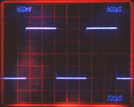
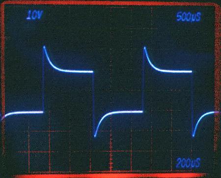
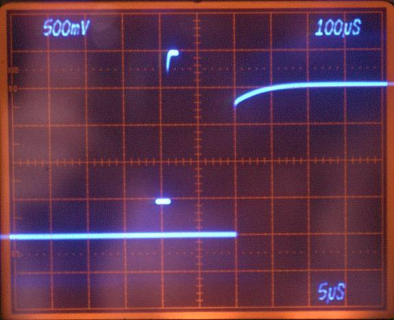
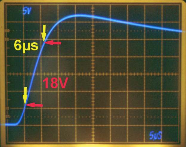
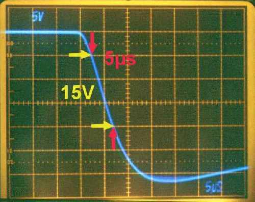
Slew Rate measurement
Slew Rate
is measured by applying a symetrical square inut voltage. The slew rate is
defined as the slope between 10% and 90% of the signal. It can be measured
either on the rising or the falling edge. Important, the square edge must
be much more faster than the excepted amplifier output response. Best
choose a square wave frequency still in the working range of the
amplifier. For audio amplifier, for example a 1 kHz with a output
amplitude of 10 volt under a less inductive 4 ohm load.
|